Table Of Contents

• Practical Example 1: Guided Shortest Paths
• So What is a metric tensor?
• Practical Example 2: Particle Alignment
• Appendix
• References and Project Files

The goal of this article is to give you a brief introduction into the world of metric tensors, and how they can be applied to artistic problems in the computer graphics context.

This article assumes you are familiar with linear algebra in the context of computer graphics.

Practical Example 1: Guided Shortest Paths

Before I get my hands dirty with any kind of maths explanation, I think seeing a practical application of what we’re going to be working towards, is important.

And the first example of how defining a metric tensor can be useful, is by guiding the output of something like Dijkstra’s algorithm,

See the Pen Untitled by Jake Rice (@tearsofjake) on CodePen.

The idea here is that we can use a metric we define, to weight the edges of an input graph such that it flows along some prescribed vector field. Which leads to really interesting and pretty outputs.

It’s worth messing around with the code pen, toggling between the metric weighted output and the non metric weighted output. I’ve also included some controls for the input noise vector field, and vector visualizers since it’s fun to play with.

So What is a metric tensor?

I will say for the purposes of this explanation, \(\boldsymbol{v}\) is a vector with a non zero length.

One way to measure the length of vectors is by taking the usual inner product (dot product) of said vector with itself \(\boldsymbol{v^T v}\), the result of this operation is the squared euclidean length of the vector, \(\boldsymbol{v^T v = ||v||^2}\).

Another way of writing this exact same operation is by inserting an identity matrix \(\boldsymbol{I}\) into the mix:

\(\boldsymbol{v^TI v = v^T v = ||v||^2}\)

However, let’s suppose that we replace the matrix \(\boldsymbol{I}\) with some arbitrary positive definite matrix \(\boldsymbol{M}\). Then if we do the same operation \(\boldsymbol{v^TM v}\) the result tells us how long of a distance \(\boldsymbol{v}\) spans, with some stretch factor from \(\boldsymbol{M}\) applied to it.

The term positive definite is doing some heavy lifting, what does that actually mean? For our purposes, \(\boldsymbol{M}\) just needs to be a matrix such that it satisfies the following statement:

\(\boldsymbol{v^TM v \gt 0}\)

for all vectors \(\boldsymbol{v}\). As long as \(\boldsymbol{M}\) does not somehow warp any vector so far as to make it return a negative value when dotted against itself, then we can say \(\boldsymbol{M}\) is positive definite.

Another property of positive definite matrices, is that their eigenvalues will always be positive. The geometric intuition here is that eigenvalues define the amount of stretch a given eigenvector will apply to a vector \(\boldsymbol{v}\) when the matrix is applied to it. In other words if we stretch space by some negative amount along a specific direction with our matrix \(\boldsymbol{M}\), then for some non zero vector \(\boldsymbol{v}\), the rule we described above, \(\boldsymbol{v^TM v \gt 0}\), will no longer be satisfied.

All of the above is an incredibly long winded way of saying, if we apply some stretching of space, we need to make sure distances remain positive no matter what.

I’m not sure if this needs to be said, but negative distances are impossible. If I got an alert that my Amazon package was -30 Miles from my house I’d throw up! I need that order of Flushable Wipes ASAP!

So to finally answer the question of what is a metric tensor, a metric tensor is the field of matrices (tensors, it lowkey does not matter) \(\boldsymbol{M}\) for all points in space that allows for defining distances or angles. For manifolds, this is usually described as the Riemannian metric.

To finally explain what we did in the Guided Shortest Paths example, rather than using euclidean distances as our edge weights for Dijkstras Algorithm, we defined a metric tensor on each edge and measured our edge distances using that instead.

The real challenge in applying the above ideas is that we need some way to actually make this tensor field. And not only that, it should hopefully be art directable in some meaningful way, so that you as an artist can focus on making interesting outputs as opposed to crunching numbers.

And lucky for us the paper “Anisotropic Geodesics for Perceptual Grouping and Domain Meshing”[0] by Bougleux et. al, proposes an incredibly easy method for defining an art directable metric tensor field, that is driven purely by a user provided vector field.

In an effort to not bore you with the nitty gritty details of their method, I want to apply the idea to another practical problem, since application is deeply important to actually internalizing things, in my humble opinion. And then in the article’s appendix I’ll spell out the method in detail.

Practical Example 2: Particle Alignment

A few months ago I saw an interesting question on twitter from Ehsan Parizi, given a random distribution of points, is there a way to organically align the particles into linear-like groups.

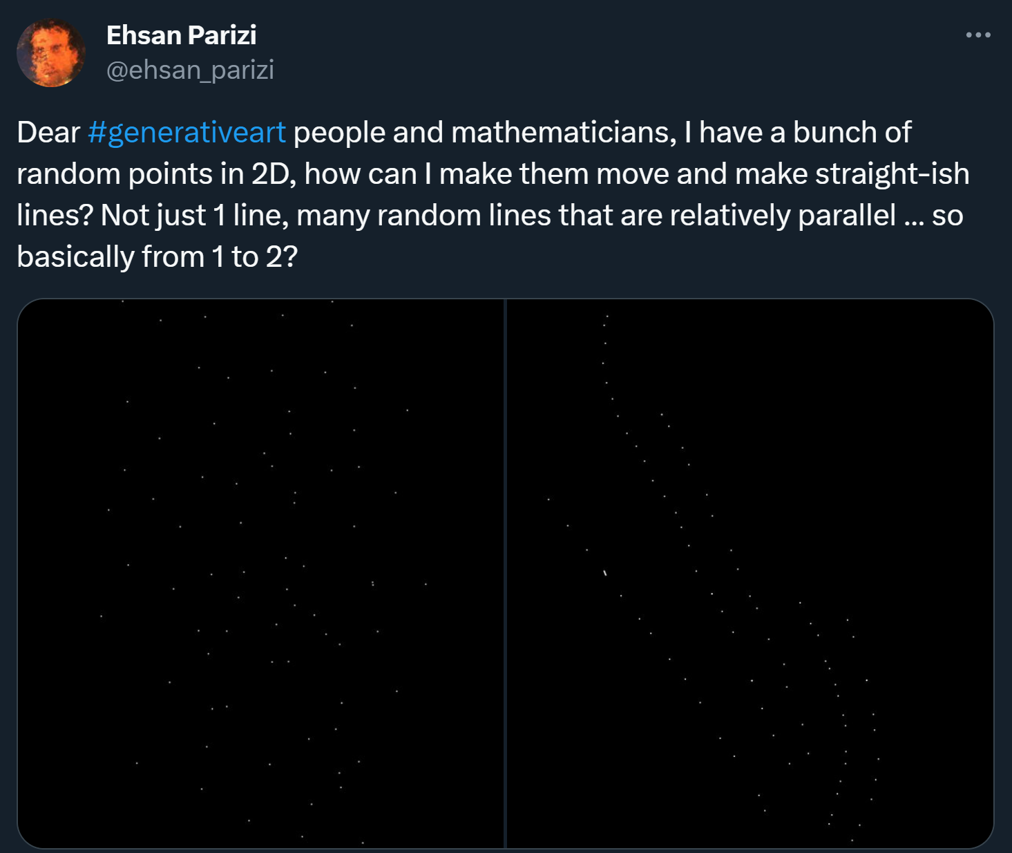
I thought this was kind of a cool problem and the first idea that jumped into my brain was to abuse what we know about weighted distances with metrics, to force oriented particles to cluster with similarly oriented particles.

See the Pen Anisotropic Weighted Particle Clustering Thingy.... by Jake Rice (@tearsofjake) on CodePen.

Sorry if the simulation runs a bit slow, Javascript is annoyingly single threaded, and WebGPU isn’t supported everywhere. And writing this as a custom WebGL thing seemed annoying. So if you want speed, I’d recommend downloading the houdini project files play with those.

The idea is at every frame of a simulation we do the following:

//dt is the time step length of the simulation (in my tests i've been doing 1/24)
//X_i is the anisotropy direction vector at each point i
//Y_i is the output anisotropy director vector at each point i

//P_i is the position of each point i
//H_i is the metric at each point i
//V_i is the velocity at each point i

//W_i is the sum of weights at each point i

//N is the maximum number of points to query

//reset temp values and compute our tensor field
for each point_i do:
    H_i = make_metric_from_vector_direction(X_i) //I will define this function at the end of the article.
    V_i = 0
    Y_i = 0
    W_i = 0

//compute our forces
for each point_i do:
    for each N nearest points_j within a euclidean radius of point_i do:
        dir_ij = P_j - P_i
        w_ij = dot(dir_ij^T * H_j, dir_ij) //distance weighted by metric
        W_i += w_ij
        Y_i += w_ij * X_j 
        V_i += (dir_ij + (X_j * -dot(X_j^T,dir_ij)) / dot(X_j^T,X_j)) * w_ij //velocity update

//integrate forces
for each point i do:
    P_i =  P_i + (V_i / W_i) * dt
    X_i = (1 - dt) * X_i + (dt) * (Y_i / W_i)

I want to briefly break down our velocity update which is a bit bizarre looking. The main crux of the idea, is that we want to avoid clumping particles together, and instead we want to align them. This means rather than sucking towards our neighbors, we want to move in a direction that will align us with the prescribed direction of that particle. To do this we use vector projection.

Often times you’ll see vector projection described as so, where you have some points \(\boldsymbol{x}\) and \(\boldsymbol{y}\), and a normal at \(\boldsymbol{y}\), \(\boldsymbol{n}\). To project \(\boldsymbol{x}\) onto the plane spanned by \(\boldsymbol{y}\) and \(\boldsymbol{n}\), you would do:

\(\boldsymbol{x_\text{projected} = x - n * ((y - x)^Tn)}\)

But again this moves \(\boldsymbol{x}\) onto the the plane spanned by \(\boldsymbol{n}\), and in our case, we want to move \(\boldsymbol{x}\) onto the infinite line passing through \(\boldsymbol{y}\), with a direction of \(\boldsymbol{n}\). We can do this by rearranging terms:

\(\boldsymbol{x_\text{projected} = y + n * ((y - x)^Tn)}\)

Our updated position is essentially the above idea, but instead of explicitly setting our position to live on this line, we take the weighted average of directions to a bunch of neighboring lines, and use that as our velocity. This gradually pushes our particles to align with each other, and creates some really interesting structures.

This update step alone, with no weighting, does cause some amount of alignment, however without the metric weighting, the particles tend to take far longer to align, and even still, they never truly converge into straight lines (in my experience).

As a brief aside, there are other ways of achieving this same particle clustering effect, one fun one is to do ray plane intersection from all the nearest neighbors with the current particle’s anisotropy direction. And then move the particle towards the geometric mean of the intersections. This converges faster than the idea I’m presenting here, but it really doesn’t have anything to do with metric tensors… Maybe in two years when I muster up the strength to write another blog post, I’ll cover that.

Appendix

In order to construct a metric tensor from some input vector field we need to do the following:

Given our vector field \(\boldsymbol{X}\) (we’ll just be using vector2s for this example, this can extend into any dimension), a tensor field at every point in space can be constructed by saying, for each vector \(\boldsymbol{u_i}\) in \(\boldsymbol{X}\), compute the matrix2 field \(\boldsymbol{M}\):

\(\boldsymbol{M_i = u_iu_i^T}\).

I would love for this to be all it takes to make this a valid matric tensor field, however these matrices have no positive definiteness guarantee. In order to force these matrices \(\boldsymbol{M}\) to be positive definite, we want to remap the eigenvalues of the matrix \(\boldsymbol{M}\) to always be positive (remember our rules for positive definiteness from above).

To do this remapping, we’ll want to decompose \(\boldsymbol{M}\) into it’s eigen vectors \(\boldsymbol{e0, e1}\) and eigenvalues \(\boldsymbol{a0, a1}\). We can then apply some remapping to \(\boldsymbol{a0}\) and \(\boldsymbol{a1}\) and reconstruct a matrix \(\boldsymbol{H}\) that approximates our original matrix \(\boldsymbol{M}\), but with the guarantee that we’re positive definite.

\(\boldsymbol{H = f(a0) * (e0e0^T) + f(a1) * (e1e1^T)}\)

where:

\(\boldsymbol{f(x) = (\text{epsilon} + |x|)^{-1}}\) for some small epsilon value that controls how extreme the anisotropy will be.

And in psuedocode form this all looks like:

function remap_values(float value, epsilon) -> float:
    return pow(epsilon + abs(value), -1)

function make_metric_from_vector_direction(vector2 u) -> matrix2:
    M = outerproduct(u,u)
    (evals, evecs) = EigenDecomp(H)
    eps = .9999
    return (remap_values(evals[0], eps) * outerproduct(evecs[0], evecs[0]) + 
            remap_values(evals[1], eps) * outerproduct(evecs[1], evecs[1]))

References and Project Files

[0]: Bougleux, Peyré, Cohen: Anisotropic Geodesics for Perceptual Grouping and Domain Meshing

Houdini Project Files